一.数据抓取 本次爬虫目标网站是中国社会组织公共服务平台。
第一步 分析网站
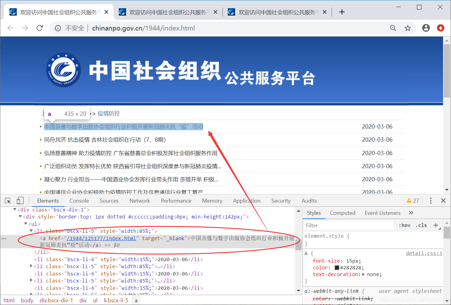
通过浏览器“审查元素”查看源代码并获取新闻的标题、URL、时间等。不同网站有不同分析方法,本文重点是文本挖掘分析。
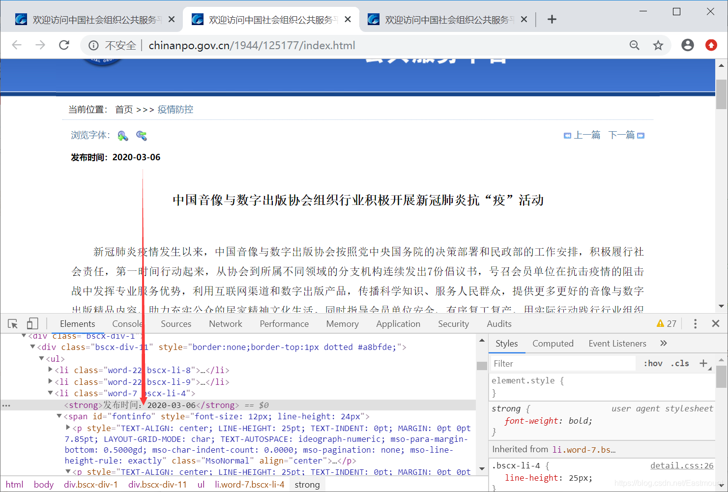
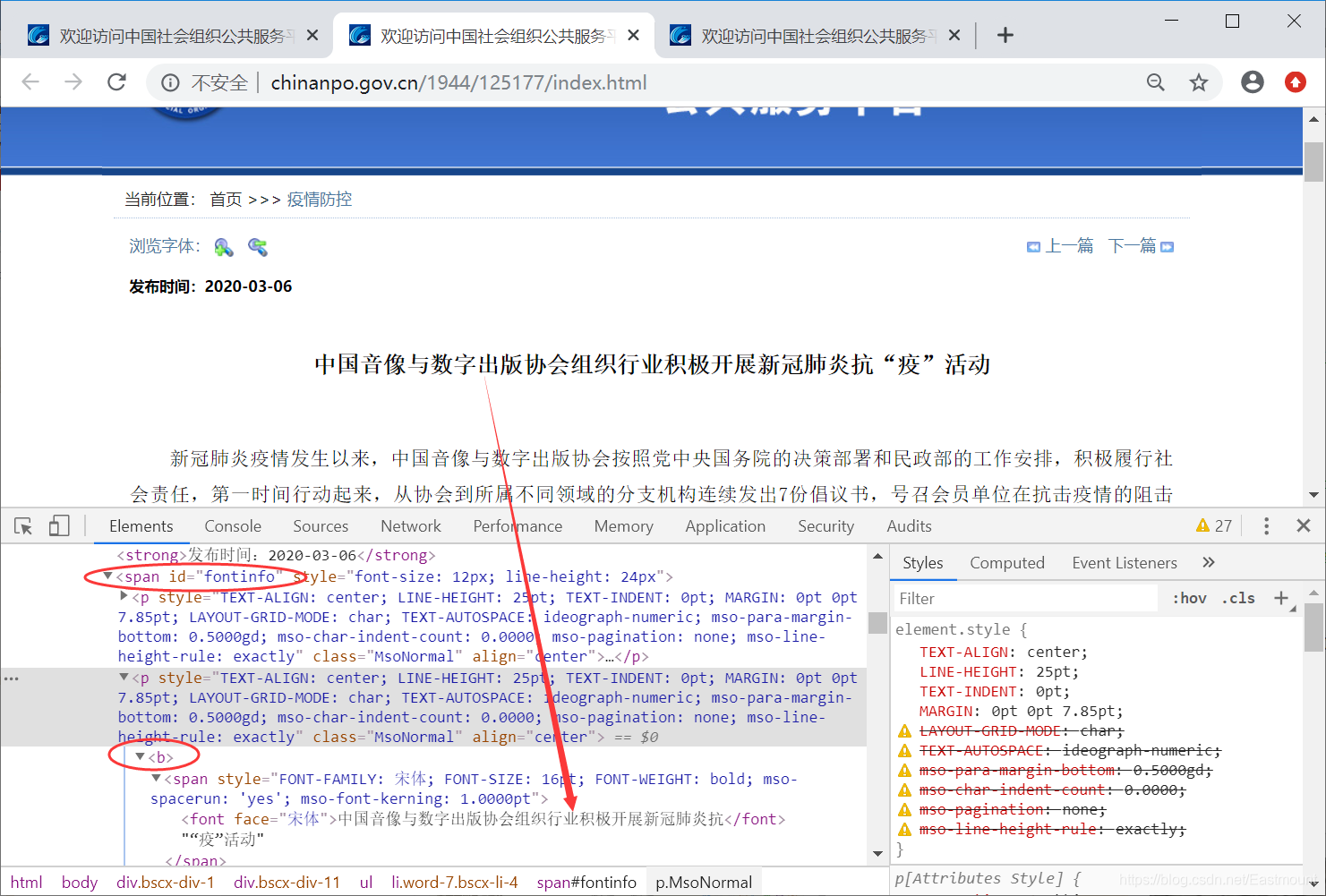
第二步,进入具体的新闻页面抓取相关的文本信息。
article_title = text_html.xpath(’//*[@id=“fontinfo”]/p[2]/b[1]//text()’)
publish_time = text_html.xpath(’/html/body/div[2]/div/ul[1]/li[3]/strong/text()’)[0][5:]
source_text = text_html.xpath(’//*[@id=“fontinfo”]/p[last()]//text()’)[0]
text_list = text_html.xpath(’//*[@id=“fontinfo”]//text()’)
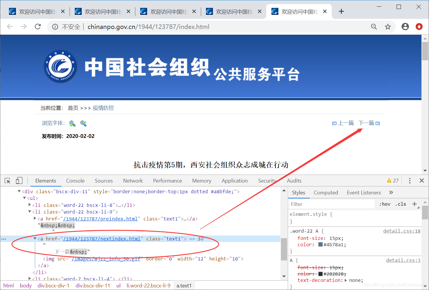
第三步,本爬虫存在一个技巧,每条新闻的URL非常相似,这里仅变换参数来抓取新闻。
我们只需要每次抓取数据时,通过“下一页”定位下次需要抓取的URL即可,核心代码为:
第四步,数据抓取完整代码如下所示。
1
2
3
4
5
6
7
8
9
10
11
12
13
14
15
16
17
18
19
20
21
22
23
24
25
26
27
28
29
30
31
32
33
34
35
36
37
38
39
40
41
42
43
44
45
46
47
48
49
50
51
52
53
54
55
56
57
58
59
60
61
62
63
64
65
66
67
68
69
70
71
72
73
import requests,re, csv, sys, timefrom lxml import htmlfrom fake_useragent import UserAgentopen ('中国社会组织_疫情防控.csv' ,'a' ,newline='' ,encoding='utf-8-sig' )"标题" , "时间" , "URL" , "正文内容" , "来源" ))def spider_html_info (url ):try :"User-Agent" : UserAgent().chrome "http://www.chinanpo.gov.cn" + text_html.xpath('/html/body/div[2]/div/ul[1]/li[2]/a[2]/@href' )[0 ]print ("next_url" , next_url)'//*[@id="fontinfo"]/p[2]/b[1]//text()' )"" .join(article_title)if title == "" :"" .join(text_html.xpath('//*[@id="fontinfo"]/p[3]/b[1]//text()' ))print ("title = " ,title)'/html/body/div[2]/div/ul[1]/li[3]/strong/text()' )[0 ][5 :]print ("publish_time = " , publish_time)print ("url = " , url)'//*[@id="fontinfo"]/p[last()]//text()' )[0 ]3 :]'//*[@id="fontinfo"]//text()' )"" .join(text_list).replace('\r\n' ,'' ).replace("\xa0" , "" ).replace("\t" , "" ).replace(source_text,"" ).replace(title, "" ) except :pass if url == 'http://www.chinanpo.gov.cn/1944/123496/index.html' :60 print ("该次所获的信息一共使用%s分钟" %useTime)0 ) else :return next_urldef main ():"http://www.chinanpo.gov.cn/1944/125177/nextindex.html" 1 while True :print ("正在爬取第%s篇:" %count, url)1 if __name__ == '__main__' :
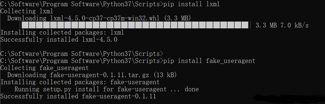
1.爬取运行截图
可能需要安装扩展包lxml和fake_useragent。
二.导入MongoDB python中csv文件中数据添加到MongoDB数据库,使用csv中的DictReader函数读取。
1.代码 1 2 3 4 5 6 7 8 9 10 11 12 13 14 15 16 17 18 19 20 21 22 23 24 25 26 27 28 29 30 31 32 33 34 from pymongo import MongoClientimport csvdef connection ():"mongodb://localhost:27017/" )None )return set1def insertToMongoDB (set1 ):with open ('中国社会组织_疫情防控.csv' ,'r' ,encoding='utf-8' ,errors='ignore' )as csvfile:0 for each in reader:1 print ('成功添加了' +str (counts)+'条数据 ' )def main ():if __name__=='__main__' :
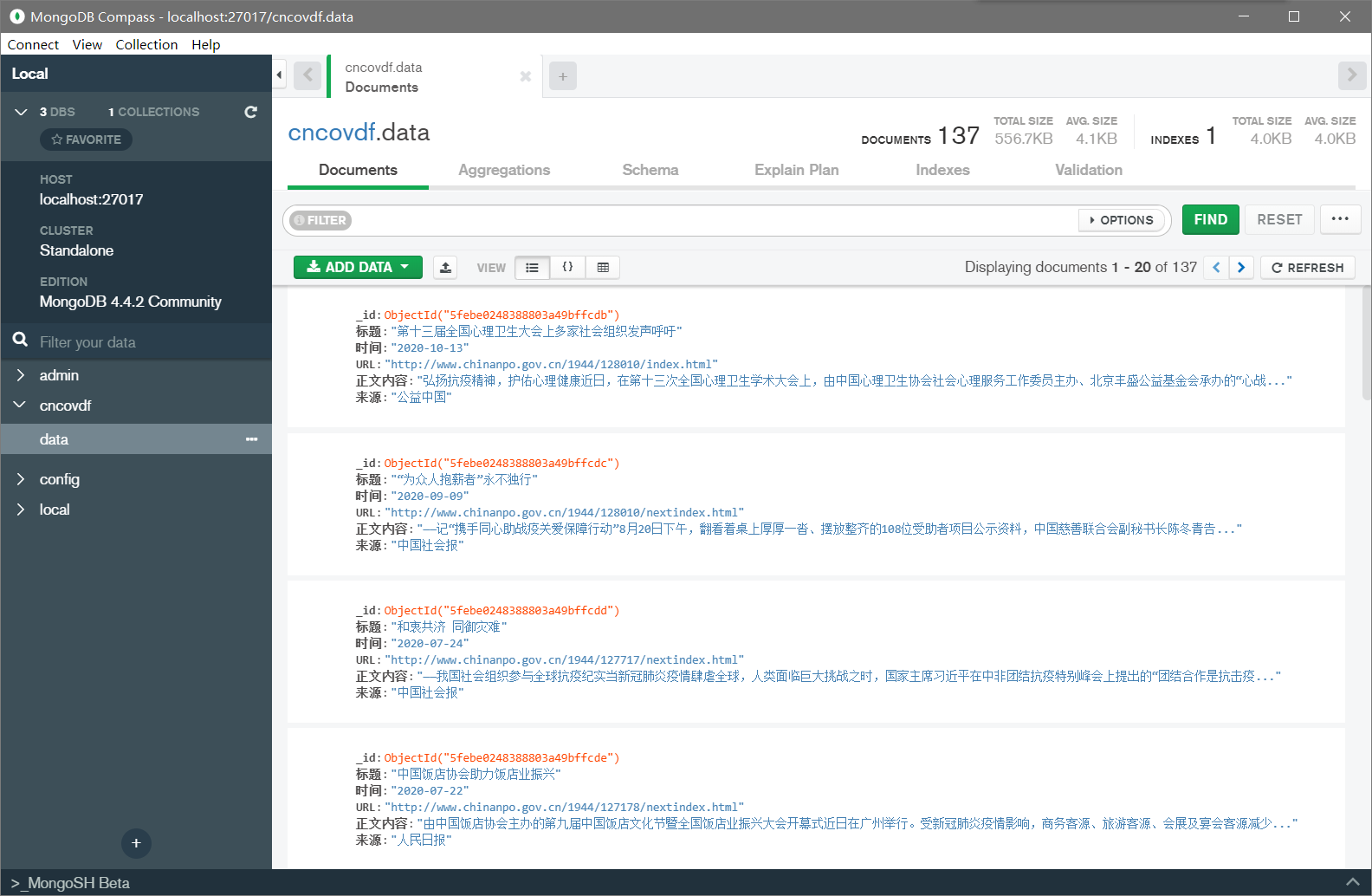
2.运行截图
三.中文分词及高频词统计 1.结巴分词 数据预处理是指在进行数据分析之前,对数据进行的一些初步处理,包括缺失值填写、噪声处理、不一致数据修正、中文分词等,其目标是得到更标准、高质量的数据,纠正错误异常数据,从而提升分析的结果。中文文本预处理的基本步骤,包括中文分词、词性标注、数据清洗、特征提取(向量空间模型存储)、权重计算(TF-IDF)等。
“结巴”(Jieba)工具是最常用的中文文本分词和处理的工具之一,它能实现中文分词、词性标注、关键词抽取、获取词语位置等功能。其在Github网站上的介绍及下载地址为:https://github.com/fxsjy/jieba
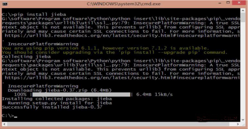
调用命令“pip install jieba”安装jieba中文分词包如下图所示。
Jieba具有以下特点:
支持三种分词模式,包括精确模式、全模式和搜索引擎模式
支持繁体分词
支持自定义词典
代码对Python2和Python3均兼容
支持多种编程语言,包括Java、C++、Rust、PHP、R、Node.js等
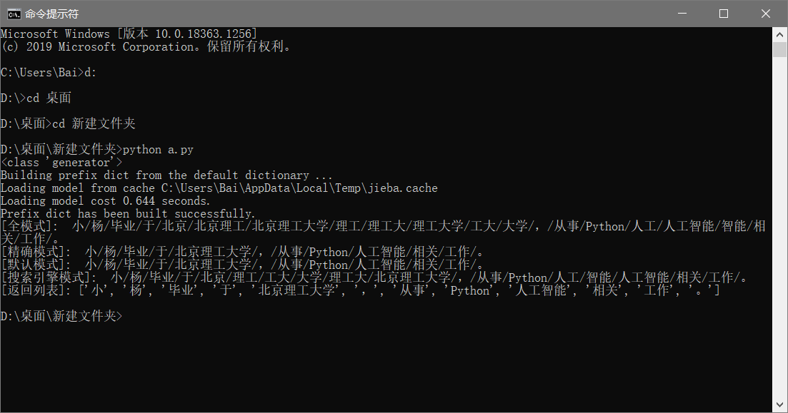
2.基本用法 首先读者看一段简单的结巴分词代码,主要调用两个函数实现。
jieba.cut(text, cut_all=True)
jieba.cut_for_search(text)1 2 3 4 5 6 7 8 9 10 11 12 13 14 15 16 17 18 19 20 21 22 23 24 25 import jieba "小杨毕业于北京理工大学,从事Python人工智能相关工作。" True )print (type (data))print (u"[全模式]: " , "/" .join(data))False )print (u"[精确模式]: " , "/" .join(data))print (u"[默认模式]: " , "/" .join(data))print (u"[搜索引擎模式]: " , "/" .join(data))False )print ("[返回列表]: {0}" .format (seg_list))
3.获取疫情文本高频词 接着我们将新闻正文文本“C-class.txt”数据进行中文分词,每行代表一条新闻,并生成对应的内容。
1 2 3 4 5 6 7 8 9 10 11 12 13 14 15 16 17 18 19 20 21 22 23 24 25 26 27 28 29 30 31 32 33 34 35 36 37 38 39 40 41 42 43 44 45 import jiebaimport reimport timefrom collections import Counter"" "" open ('C-class-fenci.txt' , 'w' , encoding='utf-8' )for line in open ('C-class.txt' , encoding='utf-8' ):'\n' )False )" " .join(seg_list))else :print (all_words)for x in all_words:if len (x)>1 and x != '\r\n' :1 print ('\n词频统计结果:' )for (k,v) in c.most_common(10 ):print ("%s:%d" %(k,v))"%Y-%m-%d" ) + "-fc.csv" open (name, 'w' , encoding='utf-8' )1 for (k,v) in c.most_common(len (c)):str (i)+',' +str (k)+',' +str (v)+'\n' )1 else :print ("Over write file!" )
输出结果如下图所示,采用空格连接的分词结果。
同时生成高频特征词,并保存至CSV文件中。
对应的特征词及词频排序如表“2020-12-29-fc.csv”所示,如果我们撰写图情论文,可以尝试建立Top50的特征词表。
四.WordCloud可视化分析 1.基本用法 词云分析主要包括两种方法:
调用WordCloud扩展包画图(兼容性极强,之前介绍过)
调用PyEcharts中的WordCloud子包画图(本文推荐新方法)
这里使用PyEcharts可视化,需要通过它来绘制词云,基础代码如下:
1 2 3 4 5 6 7 8 9 10 11 12 13 14 15 16 17 18 19 20 21 22 23 24 25 26 27 28 29 30 31 32 33 34 35 36 37 38 39 40 from pyecharts import options as optsfrom pyecharts.charts import WordCloudfrom pyecharts.globals import SymbolType'背包问题' , 10000 ),'大整数' , 6181 ),'Karatsuba乘法算法' , 4386 ),'穷举搜索' , 4055 ),'傅里叶变换' , 2467 ),'状态树遍历' , 2244 ),'剪枝' , 1868 ),'Gale-shapley' , 1484 ),'最大匹配与匈牙利算法' , 1112 ),'线索模型' , 865 ),'关键路径算法' , 847 ),'最小二乘法曲线拟合' , 582 ),'二分逼近法' , 555 ),'牛顿迭代法' , 550 ),'Bresenham算法' , 462 ),'粒子群优化' , 366 ),'Dijkstra' , 360 ),'A*算法' , 282 ),'负极大极搜索算法' , 273 ),'估值函数' , 265 )def wordcloud_base () -> WordCloud:"" , words, word_size_range=[20 , 100 ], shape='diamond' ) 'WordCloud词云' ))return c'词云图.html' )
输出结果如下图所示,出现词频越高显示越大。
核心代码为:
add(name, attr, value, shape=“circle”, word_gap=20, word_size_range=None, rotate_step=45)
name -> str: 图例名称
attr -> list: 属性名称
value -> list: 属性所对应的值
shape -> list: 词云图轮廓,有’circle’, ‘cardioid’, ‘diamond’, ‘triangleforward’, ‘triangle’, ‘pentagon’, ‘star’可选
word_gap -> int: 单词间隔,默认为20
word_size_range -> list: 单词字体大小范围,默认为[12,60]
rotate_step -> int: 旋转单词角度,默认为45
2.疫情词云 接着我们显示经过中文分词的疫情新闻文本信息,前1000个高频词的词云绘制代码如下:
1 2 3 4 5 6 7 8 9 10 11 12 13 14 15 16 17 18 19 20 21 22 23 24 25 26 27 28 29 30 31 32 33 34 35 36 37 38 39 40 41 42 43 44 45 46 47 48 49 50 51 52 53 54 55 56 57 58 59 60 61 62 63 64 65 66 67 68 69 70 import jiebaimport reimport timefrom collections import Counter"" "" open ('C-class-fenci.txt' , 'w' , encoding='utf-8' )for line in open ('C-class.txt' , encoding='utf-8' ):'\n' )False )" " .join(seg_list))else :print (all_words)for x in all_words:if len (x)>1 and x != '\r\n' :1 print ('\n词频统计结果:' )for (k,v) in c.most_common(10 ):print ("%s:%d" %(k,v))"%Y-%m-%d" ) + "-fc.csv" open (name, 'w' , encoding='utf-8' )1 for (k,v) in c.most_common(len (c)):str (i)+',' +str (k)+',' +str (v)+'\n' )1 else :print ("Over write file!" )from pyecharts import options as optsfrom pyecharts.charts import WordCloudfrom pyecharts.globals import SymbolTypefor (k,v) in c.most_common(1000 ):def wordcloud_base () -> WordCloud:"" , words, word_size_range=[20 , 100 ], shape=SymbolType.ROUND_RECT)'全国新型冠状病毒疫情词云图' ))return c'疫情词云图.html' )
运行结果如下图所示:
输出结果如下图所示:
五.TF-IDF计算及KMeans文本聚类 1.TF-IDF计算 TF-IDF(Term Frequency-InversDocument Frequency)是一种常用于信息处理和数据挖掘的加权技术。该技术采用一种统计方法,根据字词的在文本中出现的次数和在整个语料中出现的文档频率来计算一个字词在整个语料中的重要程度。它的优点是能过滤掉一些常见的却无关紧要本的词语,同时保留影响整个文本的重要字词。计算方法如下面公式所示:
$$
TF(Term Frequency)表示某个关键词在整篇文章中出现的频率。IDF(InversDocument Frequency)表示计算倒文本频率。文本频率是指某个关键词在整个语料所有文章中出现的次数。倒文档频率又称为逆文档频率,它是文档频率的倒数,主要用于降低所有文档中一些常见却对文档影响不大的词语的作用。
TF-IDF统计可视化完整代码如下:
1 2 3 4 5 6 7 8 9 10 11 12 13 14 15 16 17 18 19 20 21 22 23 24 25 26 27 28 29 30 31 32 33 34 35 36 37 38 39 40 41 42 43 44 45 46 47 48 49 import osimport timeimport pandas as pdimport numpy as npimport jiebaimport jieba.analyseimport matplotlib.pyplot as pltfrom PIL import Imagefrom datetime import datetimefrom matplotlib.font_manager import FontProperties"" for line in open ('C-class.txt' , encoding='utf-8' ):'\n' )False )" " .join(seg_list))50 ,True ,'a' ,'e' ,'n' ,'nr' ,'ns' , 'v' )) print (keywords)'词语' ,'重要性' ]).to_excel('TF_IDF关键词前50.xlsx' )'词语' ,'重要性' ]) 10 ,6 ))'TF-IDF Ranking' )range (len (ss.重要性[:25 ][::-1 ])),ss.重要性[:25 ][::-1 ])len (ss.重要性[:25 ][::-1 ])))r'c:\windows\fonts\simsun.ttc' )25 ][::-1 ],fontproperties=font)'Importance' )
输出结果如下图所示,可以看到“疫情”、“组织”、“企业”、“复工”、“社会”、“新冠”、“慈善”等都是高频词,也是大众普遍关心的主题。
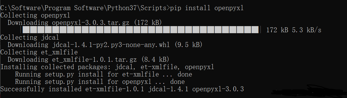
注意:可能需要安装openpyxl扩展包,to_excel()函数要用到。
2.文本聚类 同样,在Scikit-Learn包中也能计算TF-IDF权重值,此时需要用到两个类:CountVectorizer和TfidfTransformer。
(1) CountVectorizer
CountVectorizer类会将文本中的词语转换为词频矩阵,例如矩阵中包含一个元素a[i][j],它表示j词在i类文本下的词频。它通过fit_transform函数计算各个词语出现的次数,通过get_feature_names()可获取词袋中所有文本的关键字,通过toarray()可看到词频矩阵的结果。
(2) TfidfTransformer
TfidfTransformer用于统计vectorizer中每个词语的TF-IDF值。具体用法如下:
1 2 3 4 5 6 7 8 9 10 11 12 13 14 15 16 17 18 19 20 21 22 23 24 25 26 27 28 29 from sklearn.feature_extraction.text import CountVectorizer'This is the first document.' ,'This is the second second document.' ,'And the third one.' ,'Is this the first document?' ,print wordprint X.toarray()from sklearn.feature_extraction.text import TfidfTransformerprint transformerprint tfidf.toarray()
输出结果入下所示,从结果中可以看到,总共包括9个特征词,即:
同时在输出每个句子中包含特征词的个数。例如,第一句“This is the first document.”,它对应的词频为[0, 1, 1, 1, 0, 0, 1, 0, 1],假设初始序号从1开始计数,则该词频表示存在第2个位置的单词“document”共1次、第3个位置的单词“first”共1次、第4个位置的单词“is”共1次、第9个位置的单词“this”共1词。所以,每个句子都会得到一个词频向量,TF-IDF对应向量类似。
(3) 文本聚类
1 2 3 4 5 6 7 8 9 10 11 12 13 14 15 16 17 18 19 20 21 22 23 24 25 26 27 28 29 30 31 32 33 34 35 36 37 38 39 40 41 42 43 44 45 46 47 48 49 50 51 52 53 54 55 56 57 58 59 60 61 62 63 64 65 66 67 68 69 70 71 72 73 74 75 76 77 78 79 80 81 82 83 84 85 86 87 import time import re import os import sysimport codecsimport shutilimport numpy as npimport matplotlibimport scipyimport matplotlib.pyplot as pltfrom sklearn import feature_extraction from sklearn.feature_extraction.text import TfidfTransformer from sklearn.feature_extraction.text import CountVectorizerfrom sklearn.feature_extraction.text import HashingVectorizer if __name__ == "__main__" :for line in open ('C-class-fenci.txt' , 'r' , encoding='utf-8' ).readlines():print ('Features length: ' + str (len (word)))""" # 输出单词 for j in range(len(word)): print(word[j] + ' ') # 打印每类文本的tf-idf词语权重 第一个for遍历所有文本 第二个for便利某一类文本下的词语权重 for i in range(len(weight)): print u"-------这里输出第", i, u"类文本的词语tf-idf权重------" for j in range(len(word)): print weight[i][j], """ print ('Start Kmeans:' )from sklearn.cluster import KMeans2 )print (clf)print (pre)print (clf.cluster_centers_)print (clf.inertia_)from sklearn.decomposition import PCA2 ) print (newData)0 ] for n in newData]1 ] for n in newData]100 )"Cluster with Text Mining" )
输出结果如下图所示。需要注意,简单的聚类我们无法进行深入的分析,你可以理解为积极主题的一类(黄色)、消极主题的一类(黑色),也可以有其他理解,需要结合具体数据集进行分析,但其解释性始终不是很好。而真实的数据分析中会引入类标或标注,所以接着我们引入主题关键词聚类和LDA主题模型的分析,更能帮助大家理解文本挖掘和主题分析。
六.主题词层次聚类分析 1.层次聚类 层次聚类算法又称为树聚类算法,它根据数据之间的距离,透过一种层次架构方式,反复将数据进行聚合,创建一个层次以分解给定的数据集。主题词层次聚类主要调用scipy.cluster.hierarchy实现,推荐文章:层次聚类。
scipy.cluster.hierarchy.linkage(y, method=‘single’, metric=‘euclidean’, optimal_ordering=False)
层次聚类编码为一个linkage矩阵。假设代码如下,Z共有四列组成,第一字段与第二字段分别为聚类簇的编号,在初始距离前每个初始值被从0~n-1进行标识,每生成一个新的聚类簇就在此基础上增加一对新的聚类簇进行标识,第三个字段表示前两个聚类簇之间的距离,第四个字段表示新生成聚类簇所包含的元素的个数。
1 2 3 4 5 6 7 8 9 from scipy.cluster.hierarchy import dendrogram, linkage,fclusterfrom matplotlib import pyplot as pltfor i in [2 , 8 , 0 , 4 , 1 , 9 , 9 , 0 ]]print (X)'ward' )4 , 'distance' )5 , 3 ))
下面是聚类结果的可视化聚类树:
下面是返回值的解析:
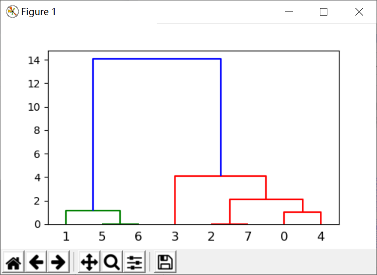
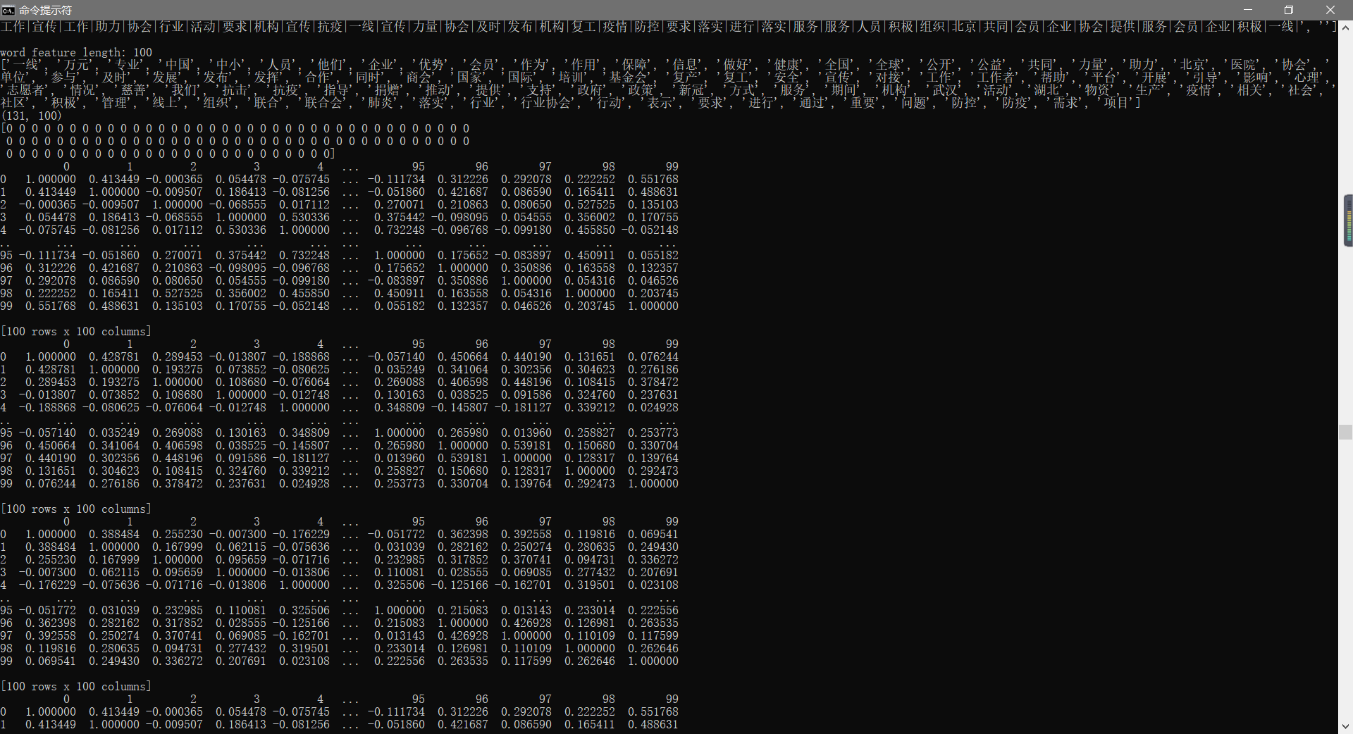
2.疫情分析 由于层次聚类绘制的树状图主题词太多,所以这里采用中文分词提取每条新闻(对应一行数据)的Top100特征词,再存储至TXT中进行层次聚类分析。完整代码如下:
1 2 3 4 5 6 7 8 9 10 11 12 13 14 15 16 17 18 19 20 21 22 23 24 25 26 27 28 29 30 31 32 33 34 35 36 37 38 39 40 41 42 43 44 45 46 47 48 49 50 51 52 53 54 55 56 57 58 59 60 61 62 63 64 65 66 67 68 69 70 71 72 73 74 75 76 77 78 79 80 81 82 83 84 85 86 87 88 89 90 91 92 93 94 95 96 97 98 99 100 101 102 103 104 105 import osimport matplotlib.pyplot as pltimport numpy as npimport pandas as pdimport jiebaimport matplotlib.pyplot as pltfrom pylab import mplfrom collections import Counterfrom sklearn.metrics.pairwise import cosine_similarityfrom scipy.cluster.hierarchy import ward, dendrogramfrom sklearn.feature_extraction.text import CountVectorizer, TfidfTransformer'font.sans-serif' ] = ['SimHei' ]"" "" for line in open ('C-class.txt' , encoding='utf-8' ):'\n' )False )" " .join(seg_list))print (all_words)for x in all_words:if len (x)>1 and x != '\r\n' :1 print ('\n词频统计结果:' )for (k,v) in c.most_common(100 ):print ("%s:%d" %(k,v))print (top_word)"" open ('C-key.txt' , 'w' )for line in open ('C-class.txt' , encoding='utf-8' ):'\n' )False )"" for seg in seg_list:if seg in top_word:"|" "\n" )print (cut_words)open ('C-key.txt' ).read()"\n" )print (list1)3 )print ("word feature length: {}" .format (len (word)))print (word)print (xx1.shape)print (xx1[0 ])print (df.corr())print (df.corr('spearman' ))print (df.corr('kendall' ))print (dist)print (type (dist))print (dist.shape)15 , 20 )) "right" , labels=titles);'Tree_word.png' , dpi=200 )
最终生成图像如下所示:
运行结果如下图所示:
注意:该方法更推荐大家在进行论文关键词共现分析、主题词聚类分析等领域。
七.LDA主题分布分析 1.LDA主题模型 文档主题生成模型(Latent Dirichlet Allocation,简称LDA)通常由包含词、主题和文档三层结构组成。LDA模型属于无监督学习技术,它是将一篇文档的每个词都以一定概率分布在某个主题上,并从这个主题中选择某个词语。文档到主题的过程是服从多项分布的,主题到词的过程也是服从多项分布的。
文档主题生成模型(Latent Dirichlet Allocation,简称LDA)又称为盘子表示法(Plate Notation),下图是模型的标示图,其中双圆圈表示可测变量,单圆圈表示潜在变量,箭头表示两个变量之间的依赖关系,矩形框表示重复抽样,对应的重复次数在矩形框的右下角显示。LDA模型的具体实现步骤如下:
从每篇网页D对应的多项分布θ中抽取每个单词对应的一个主题z。
从主题z对应的多项分布φ中抽取一个单词w。
重复步骤1和2,共计Nd次,直至遍历网页中每一个单词。
可以从gensim中下载ldamodel扩展包安装,也可以使用Sklearn机器学习包的LDA子扩展包,亦可从github中下载开源的LDA工具。下载地址详见列表所示。
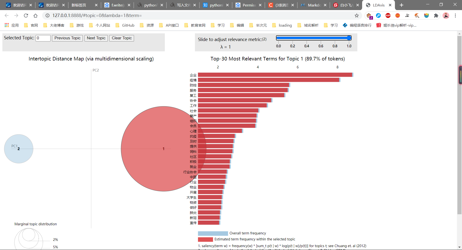
本文和之前介绍的LDA算法略有不同,它主要采用sklearn中的LatentDirichletAllocation包实现主题分布研究,并调用pyLDAvis绘制相关图形。安装过程如下所示:
2.完整代码 1 2 3 4 5 6 7 8 9 10 11 12 13 14 15 16 17 18 19 20 21 22 23 24 25 26 27 28 29 30 31 32 33 34 35 36 37 38 39 40 41 42 43 44 45 46 47 48 49 50 51 52 53 54 55 56 57 58 59 60 61 62 63 64 65 66 67 68 69 70 71 72 73 74 75 76 77 78 79 80 81 82 import pandas as pdfrom sklearn.feature_extraction.text import TfidfVectorizer, CountVectorizerfor line in open ('C-class-fenci.txt' , 'r' , encoding='utf-8' ).readlines():2000 'unicode' ,'的' ,'或' ,'等' ,'是' ,'有' ,'之' ,'与' ,'可以' ,'还是' ,'比较' ,'这里' ,'一个' ,'和' ,'也' ,'被' ,'吗' ,'于' ,'中' ,'最' ,'但是' ,'图片' ,'大家' ,'一下' ,'几天' ,'200' ,'还有' ,'一看' ,'300' ,'50' ,'哈哈哈哈' ,'“' ,'”' ,'。' ,',' ,'?' ,'、' ,';' ,'怎么' ,'本来' ,'发现' ,'and' ,'in' ,'of' ,'the' ,'我们' ,'一直' ,'真的' ,'18' ,'一次' ,'了' ,'有些' ,'已经' ,'不是' ,'这么' ,'一一' ,'一天' ,'这个' ,'这种' ,'一种' ,'位于' ,'之一' ,'天空' ,'没有' ,'很多' ,'有点' ,'什么' ,'五个' ,'特别' ],0.99 ,0.002 ) print (tf.shape)print (tf)from sklearn.decomposition import LatentDirichletAllocation2 100 ,'online' ,50 ,0 )print (lda.components_)print (lda.components_.shape) print (u'困惑度:' )print (lda.perplexity(tf,sub_sampling = False ))def print_top_words (model, tf_feature_names, n_top_words ):for topic_idx,topic in enumerate (model.components_): print ('Topic #%d:' % topic_idx)print (' ' .join([tf_feature_names[i] for i in topic.argsort()[:-n_top_words-1 :-1 ]]))print ("" )20 import pyLDAvisimport pyLDAvis.sklearnprint (data)
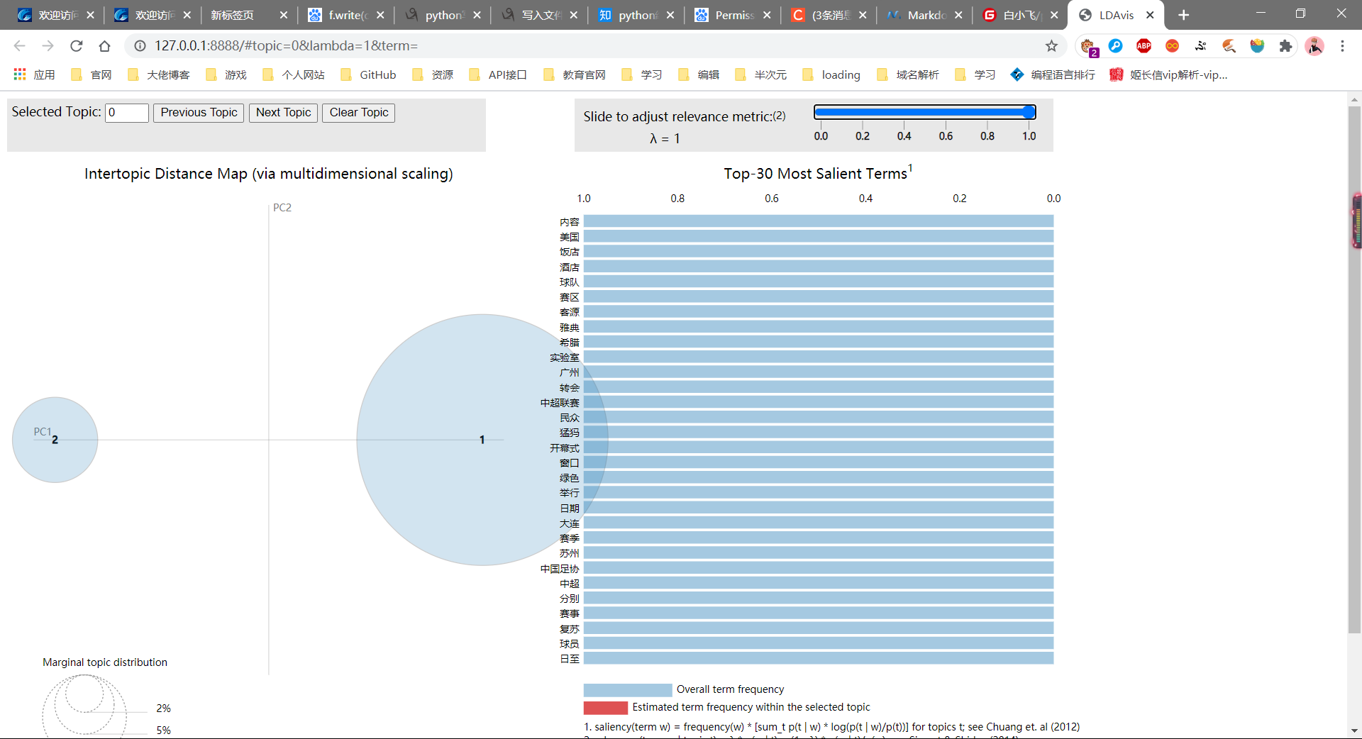
困惑度及各个主题下的关键词通过for循环显示如下,Topic1是疫情相关的主题词,Topic0是其他相关的主题。
1 2 3 4 5 6 7 8 9 10 11 12 13 14 15 16 17 18 19 20 21 22 23 24 25 26 27 28 29 30 31 32 33 34 35 36 37 38 39 40 41 42 43 44 45 46 47 48 49 50 51 52 53 54 55 56 57 58 59 60 61 62 63 64 65 66 67 68 69 70 71 72 73 74 75 76 77 78 79 80 81 82 83 84 85 86 87 88 89 90 91 92 93 94 95 96 97 98 99 100 101 102 103 104 105 106 107 108 109 110 111 112 113 114 115 116 117 118 119 120 121 D:\桌面\新建文件夹>python blog03_08_lda.py138 , 2000 )0 , 403 ) 1.0 1 , 914 ) 0.03179002916835669 1 , 916 ) 0.0234264095629235 1 , 965 ) 0.03491201537733099 1 , 873 ) 0.02309606736903826 1 , 1475 ) 0.032712252841322786 1 , 959 ) 0.030194163252955503 1 , 158 ) 0.027145424577929348 1 , 1473 ) 0.024499551271543872 1 , 1144 ) 0.058987094186498806 1 , 436 ) 0.023769709611473348 1 , 273 ) 0.030194163252955503 1 , 1662 ) 0.027145424577929348 1 , 912 ) 0.02160893613426232 1 , 1612 ) 0.03491201537733099 1 , 1942 ) 0.03491201537733099 1 , 331 ) 0.027145424577929348 1 , 712 ) 0.02884487784700509 1 , 696 ) 0.03374321119491412 1 , 1375 ) 0.03491201537733099 1 , 431 ) 0.02247058496874336 1 , 1295 ) 0.03491201537733099 1 , 210 ) 0.017702572081147446 1 , 979 ) 0.027145424577929348 1 , 1323 ) 0.03491201537733099 137 , 233 ) 0.032457418878176596 137 , 282 ) 0.02615992004194761 137 , 70 ) 0.052619347740271036 137 , 21 ) 0.04204615129757714 137 , 559 ) 0.05879281708622848 137 , 1065 ) 0.030850260311284926 137 , 1910 ) 0.02615992004194761 137 , 5 ) 0.0376578782866175 137 , 1098 ) 0.02154895843261173 137 , 1847 ) 0.022401353249301426 137 , 575 ) 0.023491381002374374 137 , 1866 ) 0.03969475253942053 137 , 1896 ) 0.07915772355142488 137 , 919 ) 0.023872748317938564 137 , 1500 ) 0.07728468461982171 137 , 753 ) 0.043373413973474426 137 , 235 ) 0.036290943551754246 137 , 1043 ) 0.02885156855169558 137 , 1576 ) 0.08423794621227862 137 , 240 ) 0.09461262585467081 137 , 1908 ) 0.12539855047313608 137 , 1435 ) 0.1301998889606912 137 , 854 ) 0.08359903364875737 137 , 1484 ) 0.09174653065996949 137 , 1044 ) 0.02885156855169558 1.47998182 1.1938479 0.93516535 ... 0.64108976 0.91951438 0.71990474 ]0.50918993 0.56496607 0.50559418 ... 0.50385102 0.50605441 0.50574252 ]]2 , 2000 )4095.2085280249858 0 0.024078 0.0 1 1 89.66411 1 -0.024078 0.0 2 1 10.33589 , topic_info= Term Freq Total Category logprob loglift403 内容 0.000000 0.000000 Default 30.0000 30.0000 1604 美国 0.000000 0.000000 Default 29.0000 29.0000 1975 饭店 0.000000 0.000000 Default 28.0000 28.0000 1865 酒店 0.000000 0.000000 Default 27.0000 27.0000 1404 球队 0.000000 0.000000 Default 26.0000 26.0000 ... ... ... ... ... ... ...1403 球员 0.093992 0.367312 Topic2 -7.2237 0.9065 886 平等 0.089363 0.349664 Topic2 -7.2742 0.9053 895 广州 0.104099 0.468188 Topic2 -7.1215 0.7660 1529 窗口 0.096892 0.421790 Topic2 -7.1933 0.7986 1304 民众 0.099578 0.576540 Topic2 -7.1659 0.5134 94 rows x 6 columns], token_table= Topic Freq Term134 1 0.810396 中国241 1 1.023200 企业255 1 1.017123 会员324 1 0.898946 做好528 1 1.054671 协会565 1 1.055105 及时715 1 1.000085 复产717 1 0.927915 复工736 1 0.886561 大学生800 1 0.942634 宣传833 1 1.133821 就业854 1 0.886084 工作919 1 0.872452 开展954 1 0.917835 心理1044 1 1.030462 抗疫1098 1 1.068630 提供1161 1 0.929940 新冠1229 1 1.078302 服务1383 1 0.851659 物业1386 1 0.894247 物资1435 1 0.981779 疫情1484 1 0.977973 社会1491 1 1.099239 社区1512 1 1.128643 积极1576 1 1.006787 组织1637 1 0.923467 肺炎1685 1 0.825705 行业1686 1 0.797830 行业协会1780 1 1.125439 赛事1908 1 1.065603 防控1910 1 0.941367 防疫1976 1 1.075012 饲料, R=30 , lambda_step=0.01 , plot_opts={'xlab' : 'PC1' , 'ylab' : 'PC2' }, topic_order=[1 , 2 ])127.0 .0 .1 :8888 / [Ctrl-C to exit]127.0 .0 .1 - - [29 /Dec/2020 22 :23 :43 ] "GET / HTTP/1.1" 200 -127.0 .0 .1 - - [29 /Dec/2020 22 :23 :44 ] "GET /LDAvis.css HTTP/1.1" 200 -127.0 .0 .1 - - [29 /Dec/2020 22 :23 :44 ] "GET /d3.js HTTP/1.1" 200 -127.0 .0 .1 - - [29 /Dec/2020 22 :23 :44 ] "GET /LDAvis.js HTTP/1.1" 200 -127.0 .0 .1 - - [29 /Dec/2020 22 :23 :44 ] code 404 , message Not Found127.0 .0 .1 - - [29 /Dec/2020 22 :23 :44 ] "GET /favicon.ico HTTP/1.1" 404 -
生成对应的图形浏览器会打开,如下图所示:
注意:LDA主题分布分析需要设置不同的主题值,这里是2,也可以是3、4、5等等。那么如何确定最佳主题数呢?困惑数又有什么用呢?如果存在语义知识又怎么处理呢?主题如何能更加准确定位呢?读者可以带着这些思考去探索。加油~
八.总结
实时数据爬取
中文文本分词及高频词提取
词云可视化分析
TF-IDF权重计算和文本聚类分析
层次聚类分析
LDA主题模型分布
参考文献: